Enter your contact information below to download the Nexus Managed IT Services buyers guide.

With the 2016 version of Excel, Microsoft has really upped the game for people who aren’t great with numbers. You can now easily use one-click access that can be customized to provide the functionality you need.
This is the first of a three-part series about using Microsoft Excel 2016 to help you identify trends, construct helpful charts, and organize information to maximize the value of your data.
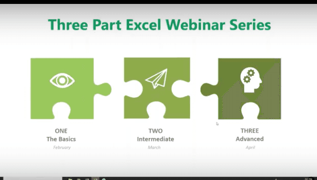
You can use Excel Worksheets and Workbooks in conjunction with programs like Microsoft Access and PowerPoint. Excel 2016 possesses many capabilities that aren’t readily apparent. That’s why we’re providing this three-part series for you.
What is Excel and how is it organized?
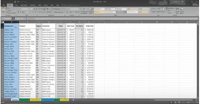
Excel is an electronic spreadsheet program that’s used to store, organize and manipulate data. You enter data into Workbooks that are made up of individual Worksheets. In the Worksheets, you enter data into cells that are organized into rows and columns. Excel data can consist of text, numbers, dates, times and formulas.
Why would you want to use Excel?
If you or your employees work with financial data, it’s a great tool to use for:
Performing calculations in Excel is only the tip of the iceberg. There’s much more you can do like creating charts and graphical layouts to make it easier to recognize trends and more easily analyze data.
Navigation
What’s great about Excel is that it has the same set up as other Microsoft products you’re familiar with. You have tabs across the top, where each tab has a corresponding ribbon with many functionalities to choose from.
The Quick Access Toolbar
The Quick Access Toolbar is a drop-down menu where you’ll find functions that you commonly use like Print and Save. You can also customize the Quick Access menu with other functions you use on a regular basis.
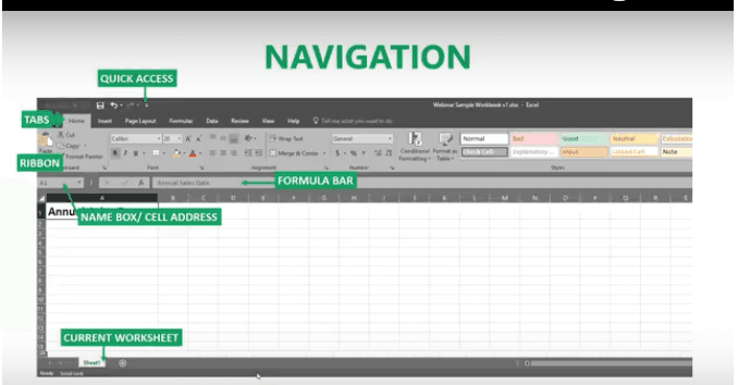
The Formula Bar
This is located underneath the ribbon next to the Name Box that shows you where your cursor is located on your Worksheet. The Formula Bar is important because it’s what calculates the math for you. Excel does the calculation and displays the answer in the cell you choose. The Formula Bar also shows you the contents of the particular cell you’re in.
Adding Data
There are three ways you can add data to your Excel Worksheet. You can:
This is great if you have a large amount of data. For example, if you have customer lists in a database, you can even pull this into Excel.
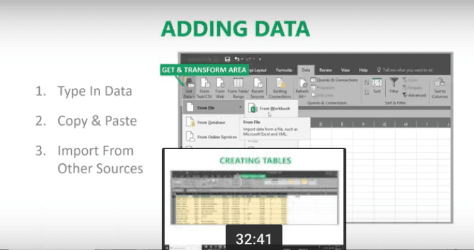
You can enter data into only one cell, into several cells at the same time, or even on more than one Worksheet at once. And, as mentioned, the data can be numbers text, formulas, dates, or times.
On your Worksheet, simply click a cell and type in the information that you want to enter. Then hit ENTER or TAB. If you typed in a date, Excel will recognize this and format it the way you’ve specified in your default settings.
Formulas
Excel computes the correct answer when you enter a formula into a cell. Once you’ve done this, it recalculates whenever you change any of the values. The way Excel knows that you’re entering a formula is by starting with an equal sign. Then you follow the equal sign with a SUM or AVERAGE.
For example, C2: =A2+B2 means that the number in C2 is what occurs when you add the numbers in A2 and B2.
You can type this in manually, but now Excel has great functionalities to help you do this. The simple way is to put your cursor in cell C2, hit = and type in A2+B2. The numbers in A2 and B2 will be added, and the SUM will be entered in cell C2.
Note: You always want to calculate using the actual cells rather than typing in numbers like 1 + 2, etc. The reason for this is so you can go back at any time and change the values in cells and the formula will calculate with the new numbers.
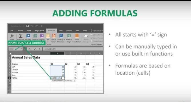
Let’s say you want to add a bunch of numbers together in your Worksheet. You can type = sum (a1:a5) in the cell where you want the answer to appear. Or you can do this and drag your mouse across the cells you want to add. Type =sum ( and drag your mouse across the cells and hit ENTER. The sum will appear in the cell without you having to typing in all the numbers! When you put your cursor on the cell, you will see the actual formula you just created.
There are many ways to do the same thing in Excel. It’s like this across all Microsoft products. You can go to the Ribbon at the top to “Auto Sum” to do the same calculation. Select a cell next to the numbers you want to add, click AutoSum on the Home tab and press Enter. Do what works best for you.
Once you create a formula, you can copy and paste it into another cell. You can also copy and paste formulas into different Worksheets as well. This can save you a lot of time.
Formatting Worksheets
With Excel 2016, you can format your Worksheets much more easily than you could before. You can use document themes throughout the Worksheets in your Workbook to present a professional and consistent appearance. You can also apply predesigned formats as well.
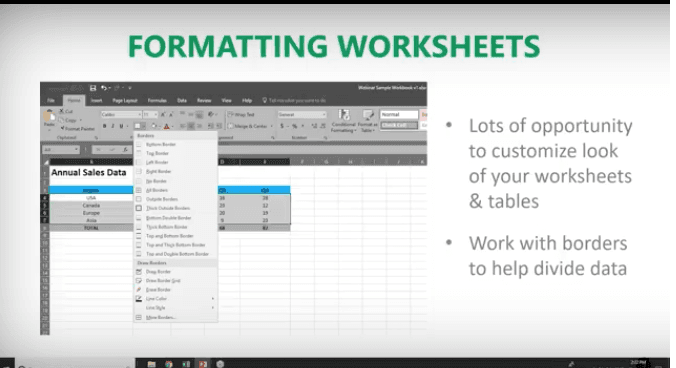
Let’s say you have a Worksheet with many rows that are hard to read. You can go in and create fill colors and more to differentiate the rows, columns, and headers to make reading much easier.
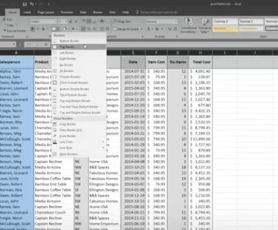
You have options to create borders around cells, rows or columns from the drop-down menu. You can also shade cells with a solid background. Don’t forget that you can change the style and types of fonts. Right-click the text, and a drop-down menu will appear where you can make these and other selections easily.
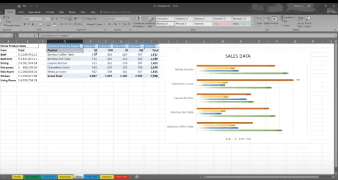
Creating Charts
If the data isn’t complex, you can easily read it, but if you have a lot of data, creating a chart will help you better analyze it. You can select specific cells, rows, and columns for your chart. One way to do this is to highlight the data and go to the top ribbon to select the type of chart you want to create.
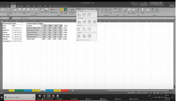
With Excel 2016, you have a “recommended charts” option. Excel will help you choose the chart that best suits your data.
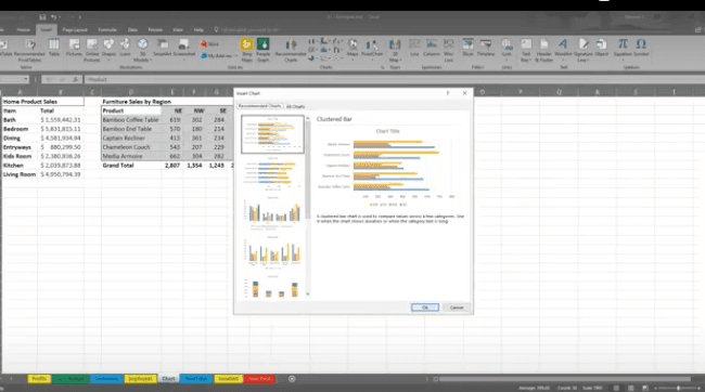
You can then go in and further customize your chart in the “Chart Tools”. You can change the color scheme, 3D effects, shading and more. If you change the data in the cells in your Worksheet, your chart will reflect the changes.
Some of the new charts in 2016 include:
Creating Tables
You may be used to creating tables in Word or PowerPoint. Some people think the format in Excel is already in a table, but it’s not; at least until you tell it to do so. If you want to do this, select your data, go to “Insert” and select “Table.”
Similar to other Microsoft products, tabs will appear to help you format your table.
Viewing Worksheets
When dealing with lots of information, it can get unruly trying to work around various rows and columns. This is where Viewing Worksheets can be helpful. You can freeze a portion of your worksheet with “Freeze Panes” to more easily view it.
You also have the ability to “split” the data to view different parts of your Worksheet. You can compare two Worksheets in the same Workbook or even in different Workbooks by viewing them side by side.
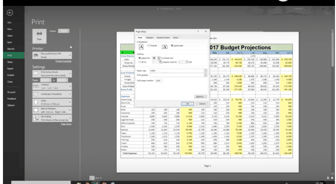
Saving and Printing
If you have Worksheets that are so large they won’t fit on one page, go to “Save As” and decide on the name, where it gets saved, and go to “Print” where you can save the file to a pdf that you can send.
You can select options for printing the entire sheet, part of it, resizing it, and more to suit your needs. Going to “Page Setup” will allow you to shrink the entire Worksheet down to a size that’s more manageable for printing.
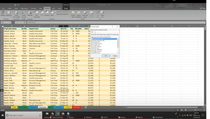
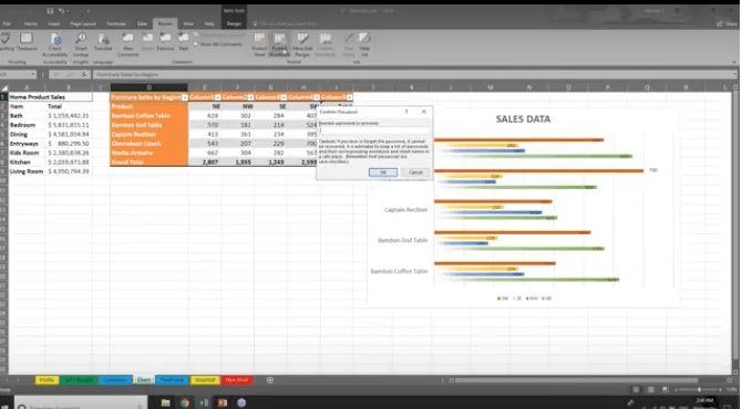
Sharing & Security
In Excel 2016 you can share Workbooks and Worksheets with others and password-protect them. The people you send them to need to know your password to open them, whether you send them via email, share them on your network, or via the cloud. From within Excel, you can designate who can access your Worksheets and Workbooks, and also whether they can edit them or not. There are a variety of parameters you can set within a Worksheet.
For example, if you want to hide employees’ salaries, you can hide this section when you share it. Or, you can let people see your data but lock it down, so they can’t change it. You can also protect your Worksheets and Workbooks to keep them secure from non-authorized users.
The Quick Analysis Tool
When highlighting data, click on the Quick Analysis button to create a chart, highlight specific cells, and much more. It doesn’t give you the functionality you’ll find in the Ribbon, but you can get things done quickly and easily with this tool.
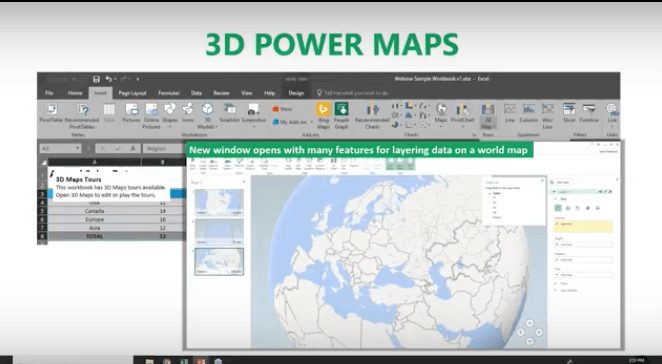
3D Power Maps
This is another new tool in Excel 2016 that lets you look at information in ways you might not have seen in the two-dimensional format. This helps you strategically create your data on a 3D map. You need latitude and longitude data to do this. You can also import your own maps into 3D Power Maps.
PivotTables
PivotTables help you analyze your Worksheet data. You can summarize, analyze, explore and present your data in just a few clicks. They are very flexible and can be adjusted to your unique needs. Note: Your data should be organized without blank rows or columns for this to work properly.
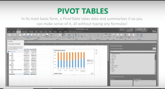
The good news is that Excel 2016 will also help you pick the best format for your PivotTables!
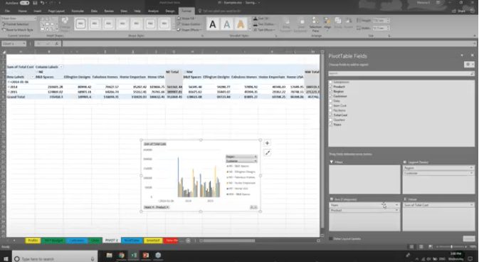
PivotCharts
PivotCharts are another great way to add visualizations to your data. You will first need a PivotTable to create a chart. Now, your PivotTable will behave like a PivotChart. When you change the information in your PivotTable, the PivotChart will also reflect this change. The PivotTable is connected to the PivotChart.
That’s it for now! For more information on using Excel 2016 like a Pro, feel free to contact the Microsoft Experts at !